 YouTube Deep Summary
![]() Extract content that makes a tangible impact on your life
Extract content that makes a tangible impact on your life
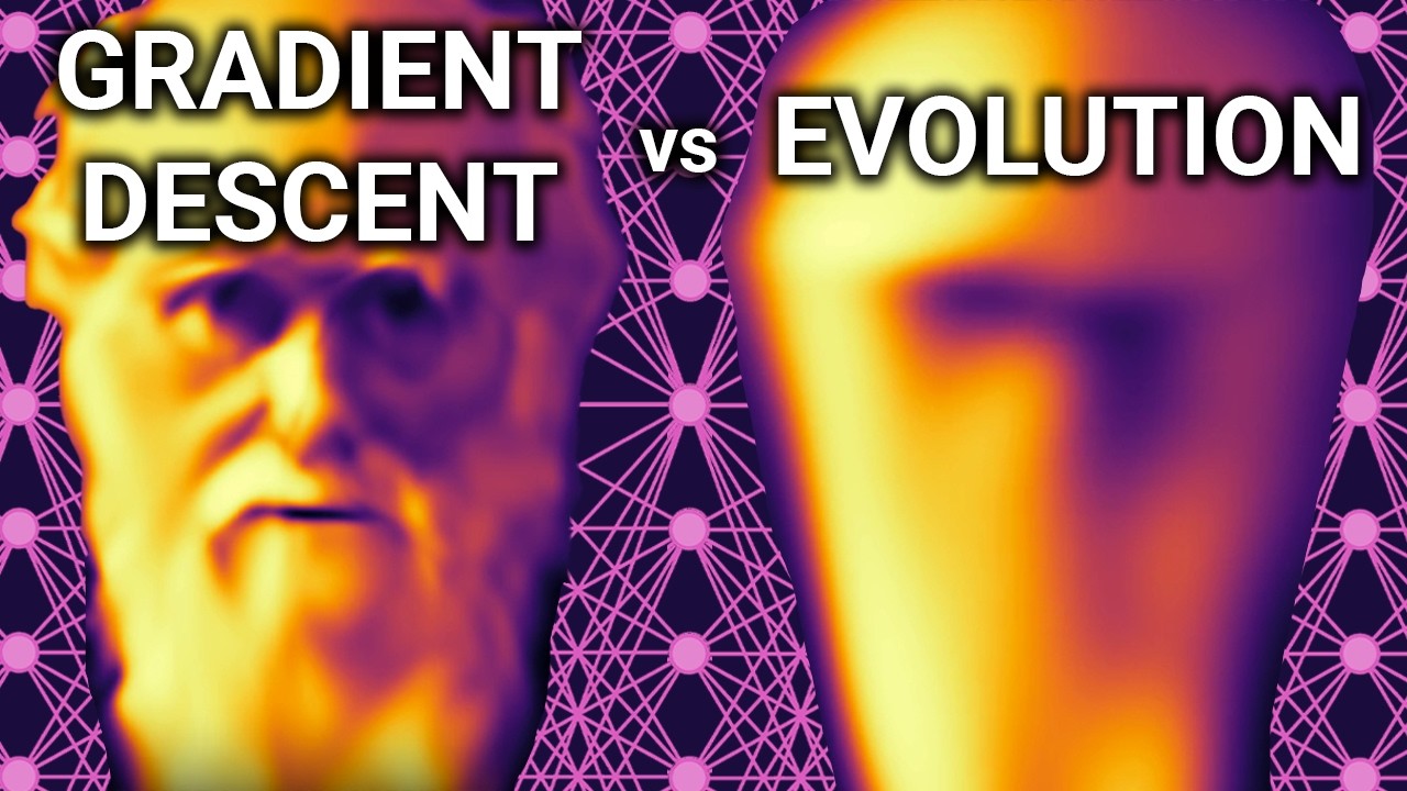
Gradient Descent vs Evolution | How Neural Networks Learn
Emergent Garden • 2025-03-01 • 23:46 minutes • YouTube
📚 Chapter Summaries (8)
🤖 AI-Generated Summary:
Overview
This video provides an in-depth explanation of how artificial neural networks learn by optimizing their parameters. It compares two optimization algorithms—stochastic gradient descent (SGD) and a simple evolutionary algorithm—demonstrating their strengths, weaknesses, and how they perform in training neural networks to approximate functions and images.
Main Topics Covered
- Neural networks as universal function approximators
- Parameter space and loss landscape visualization
- Loss functions and error measurement
- Optimization as a search problem in parameter space
- Evolutionary algorithms for neural network training
- Stochastic gradient descent (SGD) and backpropagation
- Advantages of SGD over evolutionary methods
- Challenges like local minima and high-dimensional spaces
- Hyperparameters and their tuning
- Limitations of gradient descent (continuity and differentiability)
- Potential of evolutionary algorithms beyond gradient descent
Key Takeaways & Insights
- Neural networks approximate functions by tuning parameters (weights and biases); more parameters allow more complex functions.
- Optimization algorithms search parameter space to minimize loss, a measure of error between predicted and true outputs.
- The loss landscape is a conceptual map of loss values across parameter combinations; the goal is to find the global minimum.
- Evolutionary algorithms use random mutations and selection to descend the loss landscape but can be slow and get stuck in local minima.
- Stochastic gradient descent uses gradients (slopes) to move directly downhill, making it more efficient and scalable for large networks.
- SGD’s stochasticity arises from random initialization and training on small random batches of data, which helps generalization and efficiency.
- Gradient descent is the current state-of-the-art optimizer due to its ability to scale to billions of parameters and efficiently find minima.
- Evolutionary algorithms have limitations in high-dimensional spaces due to the exponential growth of parameter combinations but can optimize non-differentiable or irregular networks.
- Increasing the number of parameters (dimensionality) can help escape local minima via saddle points, benefiting gradient-based methods.
- Real biological evolution differs fundamentally by diverging and producing complex traits, unlike convergence-focused optimization algorithms.
Actionable Strategies
- Use gradient-based optimization (SGD or its advanced variants like Adam) for training neural networks due to efficiency and scalability.
- Implement loss functions appropriate to the task (mean squared error for regression, etc.) to evaluate network performance.
- Apply backpropagation to compute gradients automatically for each parameter.
- Use mini-batch training to introduce randomness and reduce computational load.
- Tune hyperparameters such as learning rate, batch size, population size (for evolutionary algorithms), and number of training rounds to improve performance.
- Consider adding momentum or using Adam optimizer to help escape shallow local minima and improve convergence speed.
- For problems where gradient information is unavailable or networks are non-differentiable, consider evolutionary algorithms as an alternative.
- Increase network size (parameters) thoughtfully to leverage high-dimensional properties that help optimization.
Specific Details & Examples
- Demonstrated a simple 2-parameter neural network approximating a sine wave, visualizing parameter space and loss landscape in 2D.
- Used a local search evolutionary algorithm mutating parameters and selecting the best offspring to optimize networks with thousands of parameters.
- Ran evolutionary optimization on image approximation tasks such as a smiley face and a detailed image of Charles Darwin, showing slower convergence and challenges.
- Highlighted hyperparameters like population size, number of rounds, mutation rates, and their tuning impact on evolutionary algorithm performance.
- Compared evolutionary local search with PyTorch’s SGD and Adam optimizers, showing smoother and faster convergence with gradient-based methods.
- Explained Adam optimizer as an advanced variant of SGD using first and second moments of gradients for improved step size adaptation.
- Discussed the curse of dimensionality affecting evolutionary methods but not gradient descent, which scales linearly with parameters.
Warnings & Common Mistakes
- Evolutionary algorithms can get stuck in local minima and require enormous computational resources to converge on complex problems.
- Gradient descent requires the loss function and network to be differentiable; non-differentiable networks cannot be optimized with backpropagation.
- Choosing a learning rate that is too high can cause overshooting minima; too low can slow convergence.
- Ignoring the importance of hyperparameter tuning can lead to suboptimal results in both evolutionary and gradient-based methods.
- Visual comparisons of optimization results (like images) are not scientific metrics and should be interpreted cautiously.
- Overly simplistic evolutionary algorithms do not represent the state-of-the-art in evolutionary computation and thus perform worse than optimized gradient methods.
Resources & Next Steps
- The presenter’s previous videos on neural networks as universal function approximators (recommended for background).
- The free and open-source interactive web toy demonstrating parameter space and loss landscapes for simple networks.
- Reference to 3Blue1Brown’s videos for detailed mathematical explanations of calculus and chain rule in backpropagation.
- PyTorch library for implementing real neural networks and SGD/Adam optimizers.
- Future videos promised on advanced evolutionary algorithms and neural architecture search.
- Encourage experimenting with hyperparameter tuning and different optimization algorithms to deepen understanding.
📝 Transcript Chapters (8 chapters):
📝 Transcript (585 entries):
[Music] you are currently watching an artificial neural network learn in this video as we watch neural networks learn you will learn how they learn this is a continuation of my previous videos about neural networks as universal function approximators and today I will finally explain the learning algorithm itself and already there are 500 pedantic comments saying uh it's not real learning cuz it's not conscious and it's just matri multiplications and AI is neither a nor I that sounds smart yeah yeah whatever nerds nobody cares by learning I mean optimizing we will compare two different optimization algorithms for neural networks the state-of-the-art stochastic gradient descent and for contrast a simple evolutionary algorithm we will watch real neural networks learn simple functions that let us visualize the actual training process in action I will also be using a little interact web toy that I made you can play with this right now it is a free and open- Source
website I hope to provide some insight for both newbies and experts and show the similarities and differences the advantages and disadvantages of these algorithms and ultimately explain why one of them is the most optimized Optimizer again I recommend you watch my other neural network videos but in short functions are input output machines numbers in numbers out neur networks are also functions and can reconstruct or approximate any other function to any degree of precision given only a sample of its data points they are Universal function approximators and this makes them extremely general purpose for real world tasks because functions describe the world yes the network shape as a function is defined by its set of parameters the values of its weights and biases parameters are designed to be changeable tunable and different values produce different shapes more parameters let you build more complex functions with four parameters I can fit an elephant and with five I can make him wiggle his trunk this web toy has an extremely simple network with two parameters A and B which we can control down here the green line is the approximation and the blue line is the target function and data set it's a sine wave the neural Network's actual function definition is here it's using a tan H activation and as we change the values we can see this Green Point moving around down here this is parameter space the space of all possible combinations of all possible values of A and B between 5 and POS 5 it is a 2d plane where the parameters are the coordinates 2D for 2 params each point represents a different network and collectively this is the space of all possible networks with this particular architecture with two parameters wired up in this specific way note that this space would be very difficult to visualize if we had lots of parameters like hundreds this problem will haunt us throughout the video but we will keep it simple for now so given a Target function it is clear that some of these parameters fit the target function better than others we can search the space manually to find good ones but how do we automatically find the best ones this is the job of our optimization algorithm which is fundamentally solving a search problem it must search the space for the best set of parameters that produces the best approximation in order to see which is best we need a way to evaluate a network given a set of parameters tell me how well a network with those parameters
fits the target function remember that we don't actually know what the target function is we only have a sample of data points so let's take three data points from a sine wave we can now give our Network each input from the data set and ask it to predict each output and then compare the predicted outputs to the true outputs we measure the difference between these two values using what's called a loss function in this case we will use mean squared error but there are many other loss functions for different tasks we calculate loss for all predicted versus true outputs and then take the average across the entire data set which gives us a single final score for a given Network it's loss loss loss is a measure of error so lower loss is better we're playing golf here low loss means a small difference between predicted and true outputs which means you have a good approximation this big calculation can be generalized into a function the loss landscape function which takes a set of parameters as input and outputs the loss for those parameters on our current data set now remember parameter space using this function we can visit every point in this space and calculate loss for every set of parameters every Network and visualize the loss as the height of the plane at that point this is the loss landscape it tells us how good every possible Network in this space is at approximating the Target function the Green Point represents our current Network the highest points are the worst networks the lowest points are the best we want the lowest mathematically optimization simply means you are either minimizing or maximizing a function or some kind of Min maxing but we're not worrying about that in this video for minimizing you're trying to find the best inputs that produce the lowest output we are trying to minimize the loss landscape function whose inputs are parameters the data set values are not passed in as variables but rather treated as constants numbers hardwired into the function they don't change no matter what your parameters are this requires a conceptual rewiring of our neural network such that what were variables data set inputs are now constants and what were constants parameters are now variables thinking this way allows us to optimize input parameters to minimize output loss we can now search parameter space using the loss landscape as our map we can just visually look at it and see that the lowest point is here so these parameters make for the best network problem solved we're done except of course in order to show this landscape I have to generate and evaluate every possible variation of the Network in this space at least with two parameters this is easy but two parameters is nothing even on easy problems a good approximation requires hundreds of parameters which is both impossible to visualize and intractable to compute you cannot realistically generate every possible combination of 100 parameters in a 100 dimensional hyperspace and that is still very small for a neural network with that many parameters the loss landscape function can still be defined and the loss for an individual Point can be count calculated but the entire landscape can never be explicitly calculated in the way that we've done here so our optimization algorithm must make do with this limitation it must scale even with absurdly high numbers of parameters we've kept the dimensionality low so we can visualize it but our algorithm must navigate the landscape [Music] blind imagine you are near the top of a mountain range the landscape is rugged with with many Peaks and valleys the air is cold and thin and you must find your way down the mountain but there's a hitch you are blind I'm going to interview Eric Wan mayor who climbed the highest mountain in the world Mount Everest but he's gay I mean he's gay excuse me he's blind so we'll hear about that coming up okay that's you they're talking about blind and gay and stuck at the top of Lost Mountain how do you find your way down well one way you can try is to Simply step in a random Direction and if you go down commit to the step otherwise do another random Step better yet take like 10 random steps and only commit to the best one repeat this over and over this is the evolutionary way or you could just feel the slope of the ground under your feet and step in exactly the direction that it feels steepest downhill that is the gradient descent way both are hill climbing optimization algorithms step by step they climb down loss Mountain seeking the lowest point on the entire landscape the global minimum let's start with the evolutionary way random guessing and checking we'll use an algorithm known as a local search and it is just about the most Bare Bones genetic algorithm that you could ask for start with a random Network a random point and parameter space copy it and mutate the copy's parameters by adding a small random value to all or some of them this moves the point around a bit do this several times so generate a population of candidate random steps calculate loss for all and choose the one with the lowest loss for the next round and repeat repeat repeat gradually step by step its descendants descend the mountain the parameters are the Genome of the neural network and our loss function is the fitness function or anti- Fitness function as biological life seeks the highest point on the the fitness landscape we seek the lowest point on the loss landscape this website is actually performing a local search which works pretty well on this problem it can quickly find the lowest point on the landscape we say it converges on the global minimum it reaches a point where it just keeps getting closer and closer and closer it is not guaranteed to converge on the global minimum I will explain more about that in a bit either way it finds the best approximation but it still isn't a great approximation and of course it's not two parameters does not make for a very useful neural network so let's switch over to a real pytorch neural network and evolve it using a local search this network has 1,741 parameters so we can no longer observe the Lost landscape directly but we can observe the Learned function it mutates a random subset of parameters at a time and you can actually see it adjusting them as it learns the mutation rate gets smaller over time so it can hopefully learn f finer and finer details I ran this for 150 rounds each with a population of a th000 so I had to generate 150,000 networks for this footage that is a sacrifice I'm willing to make that's pretty good now let's try a more complex thing an image we'll use a smiley face refresher on how this works the network takes the pixel coordinates as input and outputs a single Pixel value two inputs one output this image is made of of every output for every pixel you treat every pixel in the Target image as a data point in your data set and approximate it every frame is a successful mutation a strict Improvement on the frame before loss can only go down or stay the same this task is harder than the previous one it takes a while but it does eventually converge now if we give it a proper image like this picture of Mr Darwin himself we can see just just how much it struggles to optimize I had to tune the algorithm quite a bit to get it to perform even decently the values that I tune the population size the number of rounds the number of neurons these values are called hyperparameters they are not learned during training but set beforehand you can tune them by hand as I have or use a meta optimization algorithm to find good hyperparameters we're not doing that here so it seems to have hit a wall this may be due to the local search getting stuck in one of the many shallow valleys that are still high up on loss Mountain these are local Minima and they are where hill climbers go to die our local search cannot climb up and out it can only go down loss always goes down likewise real genetic fitness always goes up and it too can get stuck on low hilltops it can only make do with what it's got it cannot go back to the drawing board our algorithm might be getting stuck in one of these local Minima but if you just keep running it it does keep improving very slowly gradualism baby we could improve this by keeping a diverse population of good candidates throughout the entire run mixing their parameters with crossover mutations we could be mutating the neural architecture itself and other hyper parameters along the way I will explore these in a future video but for now we must move on a local search works
pretty well if you have a billion years but if you don't want to die before it converges you will need something like gradient descent stochastic gradient descent or SGD stochastic means it involves Randomness descent it's going down the hill and the gradient is our secret weapon the gradient is a vector a list of numbers each holding the slope of the corresponding parameter on loss Mountain if you have two parameters you have two gradient values Collective ly they make a line seen here actually that is the line tangent to the surface which is not quite the same thing but it includes the gradient the gradient Vector points in the direction of the steepest slope from the current position on the landscape give it a negative sign and it points to the steepest slope downhill the gradient is our compass on L Mountain it is the slope of the ground that we can feel under our feet calculating it requires some calculus multivariable calc I defined the Lost landscape function a bit more generally here we need to take its derivative with respect to each parameter and we can do this because our lost landscape function is always well defined even though our Target function is unknown so we start by using the derivative law known as use wolf from Alpha and here's the derivatives go watch three blue one Brown's video for the mathy math there's a chain rule in there somewhere that gives us a partial derivative function for each parameter which combined gives us our great radiant Vector these functions tell us how loss changes as each parameter changes this gets complicated for large neural networks but it can be fully automated now we can calculate the gradient for any point and step directly towards the steepest downhill Direction by simply subtracting the gradient from the parameters except that's probably too much you will overshoot it you want to scale the gradient down with a learning rate hyperparameter something like 0 2 the gradient tells you the optimal Direction but not the optimal step size you're still blind you don't know what the function will look like in the next step there are clever ways of choosing better step sizes we'll talk more about that later just know that because the gradient tells you the best direction to step there is no guessing and checking this is a crucial Advantage we once again randomly initialize our Network and evaluate loss with a forward pass then we go back throughout the entire network calculate the gradient for each parameter and apply the step which moves the point this is the backwards pass AKA back propagation and repeat this results in a much smoother more precise stepping algorithm than Evolution it is still a gradualistic hill climber but more direct and less Spazzy although it can get jumpy on steep slopes it is not guaranteed to always reduce loss the stochastic part comes from the random initialization but also something called random batching rather than training on the entire data set all at once we train on small random subsets of the data called batches we go through every batch in the data set taking a step for each and then randomize the batches for the next pass you can simulate this effect
with simulate batching which purely randomizes the data on every step because the landscape is defined by the data set it changes with every batch but in the long run these variations will average out to the same landscape mathematically it is equivalent to train on the entire data set all at once as it is to train on small random batches though in practice hyperparameters must be tuned batching is extremely useful because it allows us to spread out the expensive back propagation algorithm over more compute time so let's train a real network using SGD this is using the exact same architecture as our search but this time with pytorch's SGD Optimizer this works good it is smoother than the local search and able to refine details to get a slightly lower loss if we train it on an image we can see that it is also smoother and really pretty looks like a candle and be aware that this visual comparison is not scientific or Fair we're just eyeballing it though SGD did take significantly less compute time to end up with a lower loss but for the image of Darwin we seem to run into a similar problem it converges very slowly and not very well actually worse than the local search again we might be getting stuck in local Minima which are just as much of a problem for gradient descent as Evolution to help we can add momentum to the final step which helps it roll out of little goalies but we've actually already been using momentum a much more radical Improvement comes from using a variant of SGD called atom atom is basically momentum on steroids it improves upon the final step size by using the first and second moments of the gradient I won't explain more about Adam but I will sing its Praises atom rocks it makes the training process way more efficient way faster and ultimately more capable the final learned functions are much more precise hello Mr Darwin looking a little creepy today now remember that these are all
generated with the exact same neural architecture just with different parameter values discovered by different [Music] algorithms there is another unintuitive way to escape local Minima scale up add more parameters which adds more Dimensions to the Lost landscape what is a minimum in one dimension maybe a maximum in another dimension this is a saddle point and it means that there is another way downhill research has shown that as you increase the dimensionality of parameter space it becomes less and less common to find true local Minima where not a single parameter can be improved on the hyperdimensional Lost landscape There is almost always another way down the mountain gradient descent is well poised to take advantage of this the gradient will usually point to the optimal direction to escape the wouldbe local Minima evolutionary algorithms can can benefit from this but they're not able to take full advantage because they must guess at parameters to mutate I.E directions to travel they are precipitously less likely to guess the right direction as the number of directions grows this is a more General problem with the evolutionary approach as you scale up the number of parameters parameter space grows exponentially it becomes explosively unlikely that you will guess the right values to mutate you will have to generate a lot of failed networks however note that it never becomes impossible just very improbable given enough time improvements will still accumulate it just might take literally billions of years we meet the curse of dimensionality again it has killed many other optimization algorithms here too the primary and unique advantage of gradient descent is scale no matter how many parameters you have you can always compute the gradient in linear time and need take only one step in the optimal Direction This lets you take advantage of massive neural networks with billions of parameters without exploding the number of computations it is the blessing of dimensionality and it is why gradient descent is the state of the art but this video is deeply unfair to evolutionary methods I am comparing a heavily optimized gradient descent implementation with a homegrown own dumb guy baby time local search I will definitely make a follow-up video on The state-of-the-art evolutionary methods I think there may be untapped advantages to algorithms other than gradient descent the main limitation of gradient descent is that to calculate the gradient it must be that the Lost landscape function the loss function and the neural network itself are continuous and differentiable or connected and smooth no holes no breakes no gaps no Jagged edges and no weird fractally bits that you can't differentiate the gradients must flow this applies to activation functions too like the reu uh this Jagged point is not differentiable but we'll just say its derivative is one and this works perfectly fine in practice what are you going to do about it math nerd however you cannot back propop through a binary step function like this but you can evolve it pretty neat and you can use it for images too and make some really creepy looking smiley faces you can't do this with gradient descent it is possible to evolve very weird neural networks that are broken Jagged or fractally that you can't train with gradient descent and this might be useful it's a neat idea and it makes an interesting image but this is not really a better approximation there is a common view that evolution is just an inferior optimization algorithm and well that is true to some extent there's a reason we don't train language models with genetic algorithms but I do think this view is missing something important true biological evolution has something that none of these algorithms have even the genetic ones if you actually ran any of these programs for a billion years you'd end up with just a better and better approximation if you run true biological evolution for a billion years you end up with eyes and wings and brains and pill bugs Evolution diverges not just converges there's a lot more to say here but alas we're outside the scope of the video right now gradient descent is the most optimized Optimizer by far it is the best tool for the job and its scales which turns out to be kind of a big deal large language models trained with gradient descent helped write the code and check the script for this video it's cool that this algorithm can encode some weird understanding of itself into the very neurons that it trains don't worry the script was human written and human fact checked too I don't really like the way AI writes and I always use human music check out my music guys they're great okay video's over get out of here